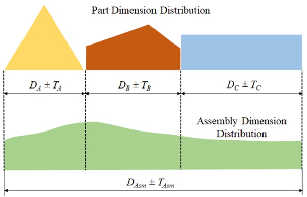
Engineers use two main methods for tolerance stacking. While the main function of either of these is the same, some key differences between them make them suitable for specific situations.
Worst Case Tolerance Analysis
The worst case tolerance stack analysis is the simpler of the two. It assumes that all features are at their maximum deviation levels, which is the ‘worst-case scenario’ for a manufacturer.
While this is an unlikely event in a real production environment, the worse case technique is adopted when the stakes are high. Especially for high-accuracy parts in industries like aviation and medicine.

For a part with n features and bilateral tolerances, the formula to find the total variation is:

The worse case method guarantees that all parts will be within tolerance and achieve the desired engineering fit. However, this confidence comes at the cost of tighter tolerances. Due to this, it is more suitable for low-volume production as the likelihood of manufacturing parts within tolerance gets lower as the number of parts grows.
Example of Worst Case Tolerance Analysis
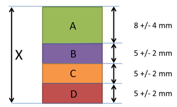
Tolerance stacking can be involved and difficult to comprehend. Thus, we present a simple tolerance stack up example to drive the point home. The figure below shows a tolerance stack with multiple features, each having its dimension and tolerance. The goal is to calculate X, the total assembly tolerance based on the worse case principle.

In the worse case tolerance stacking, the nominal dimension and tolerance are the sum of feature dimensions. Hence, X is calculated as:
|
Element |
Nominal |
Tolerance |
|
A |
8 |
±4 |
|
B |
5 |
±2 |
|
C |
5 |
±2 |
|
D |
5 |
±2 |
|
Assembly (X) |
23 |
±10 |
Therefore, X = 23 ± 10
Statistical Tolerance Analysis / RSS – Root Sum-Squared
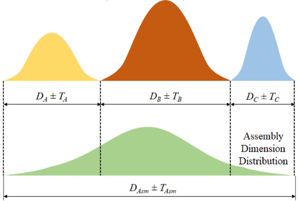
The statistical tolerance stack analysis method takes a slightly more realistic and methodical approach to tolerance stacking. It uses statistical analysis to estimate the probability distribution of deviations in each tolerance dimension.
For this, the basic hypothesis is that each dimension will be different. Some will be less off, some more, exactly like it is in a real factory. Consequently, it is widely applicable in mass production environments where a small number of errors are acceptable.
After calculating these individual probability distributions, it adds them up to compute the probability of the overall part tolerance, which gives a reasonable estimate of how many parts are expected to fail the quality tests.
It utilizes various statistical techniques, but the Root Sum Squared (RSS) method is by far the most popular, which assumes a normal distribution for the dimensional deviations.

The formula to calculate the assembly tolerance, Tasm, is:

Example of RSS Tolerance Analysis
To understand statistical tolerance stacking, let us use the same example. The nominal X dimension will remain the same at 23. The tolerance is calculated using the RSS formula.

Therefore, using RSS, X is 23 ± 5.29.


